Ma Jin, Zheng Xiangdong. Comparisons of boundary mixing layer depths determined by the empirical calculation and radiosonde profiles. J Appl Meteor Sci, 2011, 22(5): 567-576.
Citation:
Ma Jin, Zheng Xiangdong. Comparisons of boundary mixing layer depths determined by the empirical calculation and radiosonde profiles. J Appl Meteor Sci, 2011, 22(5): 567-576.
Ma Jin, Zheng Xiangdong. Comparisons of boundary mixing layer depths determined by the empirical calculation and radiosonde profiles. J Appl Meteor Sci, 2011, 22(5): 567-576.
Citation:
Ma Jin, Zheng Xiangdong. Comparisons of boundary mixing layer depths determined by the empirical calculation and radiosonde profiles. J Appl Meteor Sci, 2011, 22(5): 567-576.
Mixing layer is one typical type of atmosphere boundary layer, and it is named after strong vertical mixing which leads to the nearly constant variables, such as potential temperature and water vapor in this layer. The depth of mixing layer is an important parameter to identify features of thermodynamics and atmospheric dynamics in the boundary layer, and also a key to monitor the air quality. Mixing layer has very distinct daily variation as different meteorological conditions and synoptic processes largely influence the structure of boundary layer. Mixing layer becomes thicker under clear sky conditions, while remains physically stable and almost invariant during a single day under cloudy or raining weather conditions. Therefore, measurements and calculation of mixing layer depth are worth studying.The depths of mixing layer at 14:00 of Beijing, Longfengshan, Lin'an, Aletai, Sanya, Xining and Tengchong are compared using two kinds of datasets: The Nozaki empirical method and the radiosonde observational data reduced by vertical profiles of potential temperature and refractivity. It shows that the two observational depths are in good agreement, and the radiosonde measurements of mixing layer can be seen as criteria in the comparison with the Nozaki empirical method. Few bad linear correlation points of mixing layer depth from potential temperature profiles and refractivity profiles indicate that depth of mixing layer determined by refractivity profiles sometimes cannot find out the actual mixing layer, possibly due to dramatic variation of refractivity profiles under stable atmosphere vertical structure conditions.The comparisons illustrate that the Nozaki method may reflect the daily variations of mixing layer as those shown in observational dataset. However, the Nozaki method underestimates mixing layer depth when the mixing layer is above 2000 m. On the contrary, it overestimates mixing layer depth when the mixing layer is lower than 1000 m. Nozaki method also overestimates mixing layer depth at the sites (Beijing, Longfengshan, Aleitai, Xining) located at higher latitudes, but underestimates mixing layer depth in the sites (Sanya, Lin'an, Tengchong) at lower latitudes. Errors of Nozaki method are smaller under cloudy (total cloud amount is about 3—7) weather conditions, while larger in clear days. The lack of considering terrain effect and the simplifying of physical process maybe sources of comparative error of Nozaki method. These results suggest that the empirical determination of mixing layer depth need more subtle consideration before extensive use.
Fig.
2
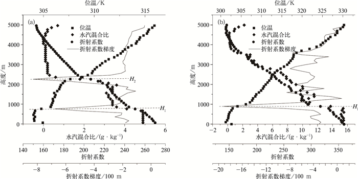
Typical refractivity profiles to identify mixing layer depth (H1 denotes mixing layer depth; H2 denotes residual layer depth) (a) in Aletai on 9 May 2005, (b) in Sanya on 19 April 2004
Basha G, Ratnam M V.Identification of atmospheric boundary layer height over a tropical station using high resolution radiosonde refractivity profiles: Comparison with GPS Radio occultation measurements. J Geophys Res, 2009, 114, D16101, doi: 10.1029/2008JD011692.
[3]
Hennemuth B, Lammert A. Determination of the atmospheric boundary layer height from radiosonde and lidar backscatter. Boundary-Layer Meteorology, 2006, 120:181-200. doi: 10.1007/s10546-005-9035-3
[4]
Shaw W J, Pekour M S, Coulter R L, et al.The daytime mixing layer observed by radiosonde, profiler, and lidar during MILAGRO.Atmos Chem Phys Discuss, 2007, 7: 15025-15065. doi: 10.5194/acpd-7-15025-2007
Holzworth G C. Mixing Heights, Wind Speeds and Potential for Urban Air Pollution Through Contiguous United States. AP-101, US EPA.
[16]
Holzworth G C. Mixing depths, wind speeds and air pollution potential for selected locations in the United States. J Appl Meteorology, 1967, 6:1039-1044. doi: 10.1175/1520-0450(1967)006<1039:MDWSAA>2.0.CO;2
[17]
Nozaki K Y. Mixing Depth Model Vsing Hourly Surface Observations. Report 7053, USAF Environmental Technical Applications Center, 1973.
[18]
Cheng S Y, Huang G H, Chakma A, et al. Estimation of atmospheric mixing heights using data from airport meteorological stations. J Environ Sci Health, 2001, 36(4): 521-532. doi: 10.1081/ESE-100103481
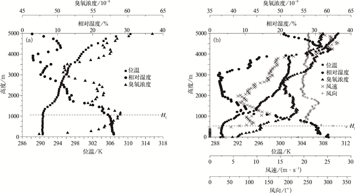
Figure 1. Typical potential temperature profiles to identify mixing layer depth (H1 denotes mixing layer depth)
Figure 2. Typical refractivity profiles to identify mixing layer depth (H1 denotes mixing layer depth; H2 denotes residual layer depth) (a) in Aletai on 9 May 2005, (b) in Sanya on 19 April 2004
Figure 3. Comparison of mixing layer depths determined by potential temperature and refractivity profiles, respectively
Figure 4. Mixing layer depths determined by potential temperature, refractivity profiles and Nozaki method at 7 sites
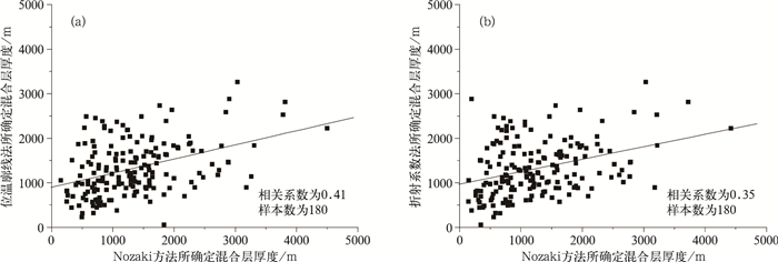
Figure 5. Comparison of mixing layer depths determined by Nozaki method and radiosonde profiles
Figure 6. Differences of mixing layer depths categorized by cloud cover of 7 sites


 DownLoad: